People usually talk about the race to the bottom in artificial intelligence as a bad thing. But it’s different when you’re discussing loss functions.
Loss functions are a crucial but frequently overlooked component of useful artificial intelligence (AI), and they’re all about getting to the bottom — albeit of a literal curve on a graph — as quickly as possible. When training an algorithm to automate tedious data analysis, such as looking for specific features in millions of photographs, you need a way of measuring its performance. That’s the ‘loss function’: it measures an algorithm’s error relative to the ‘ground truth’ of the data — information that is known to be real or true. Then you adjust the algorithm’s parameters, rinse and repeat, and hope the error is smaller next time. “You’re trying to find a minimum: the point where the error is as small as possible — hopefully zero,” says Anna Bosman, a computational-intelligence researcher at the University of Pretoria.
Dozens of off-the-shelf loss functions have been written. But choose the wrong one, or just handle it badly, and the algorithm can lead you astray. It could blatantly contradict human observations, make random fluctuations (known as experimental noise) look like data, or even obscure the central results of an experiment. “There are lots of things that can go wrong,” Bosman says. And worst of all, the opacity of AI means you might not even know that you’ve been misled.
That’s why a growing number of scientists are abandoning ready-made loss functions and constructing their own. But how do they get it right? How do you make a home-made loss function your go-to tool and not a time-swallowing mistake?
Error assessment
Table of Contents
Machine-learning algorithms are generally trained on annotated data, or by being told when they get the answer wrong. Loss functions provide a mathematical measure of wrongness, but there are multiple ways to quantify that.
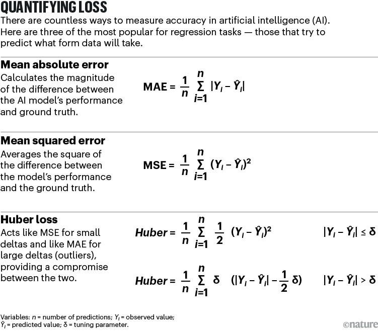
‘Absolute error’ functions, for example, report the difference between the algorithm’s prediction and the target value. Then there’s mean squared error: square the differences between your predictions and the ground truth, and then average them out across the whole data set.
Mean squared error is a simple, straightforward and proven approach that works well when errors are relatively small and consistent. But it can be problematic if your data are full of outliers, because the algorithm amplifies their impact. A loss function called pseudo-Huber (a smooth approximation of an approach called the Huber loss function) considers whether each data point’s error is large or small, providing a compromise between the mean squared error and absolute error loss functions.
Absolute error, mean squared error and Huber are most useful for regression analysis, which uses past data on continuous variables such as height or weight in a population to predict what shape future data sets will take (see ‘Quantifying loss’). Classification tasks, by contrast, answer questions such as what type of object something is and how many of them are in the data set. In this case, the machine-learning algorithm determines the probability that an object belongs to a particular class — how likely it is that a particular collection of pixels represents a dog, for example. The most useful loss functions include cross entropy, a measure that compares probability distributions related to the model’s output and the real-world value (also known as maximum likelihood), and hinge loss. The latter finds the curve that is the farthest possible distance from every data point, providing the cleanest possible decision about which category a data point falls into.

These generalized loss functions are not always the best option, however. Take Arjun Raj’s experience, for example.
A geneticist at the University of Pennsylvania in Philadelphia, Raj uses fluorescence microscopy to quantify gene expression in single cells. In these experiments, each RNA transcript is a discrete spot in an image: the trick is to count the spots and assign them to the correct cell. Finding the spots — which are two or three pixels across — is trivial for a human. “One summer, I had a high-school student working with me who had never seen these images, and I was able to teach him how to perfectly annotate the images within two minutes,” says William Niu, a former undergraduate student in Raj’s laboratory.
Unfortunately, the lab generates data sets that might represent thousands of fluorescent spots in millions of cells, too many to analyse by hand. Even more unfortunately, the analysis is much harder for machines than it is for humans. When Raj and his colleagues tried to automate the process, they found that no known loss function could return a reliable result.
The problem mainly came down to ‘class imbalance’, Raj says: when spots are few and far between, the algorithm might think that it is performing well if it simply labels every pixel as ‘not-spot’. But that gives a catastrophically high false-negative rate. “You could make a really ‘good’ classifier that just said there’s no spots in this image because 99.9% of the time, there are no spots,” Raj says. “It’s very, very accurate in some sense, even though it’s basically doing nothing useful at all.”

AI and science: what 1,600 researchers think
Niu, Raj and others in their lab worked together to translate their understanding of the issues into a loss function called SmoothF11. F1 is a metric that balances false negatives against false positives. However, the mathematical function behind F1 cannot be differentiated, which means it can’t be used to train a neural network, because it lacks a way to minimize the algorithm’s error. SmoothF1 approximates the F1 score in a way that compensates for class imbalance while allowing the algorithm to find its way to the bottom of the error slope. The team then used this function to drive a spot-detection algorithm called Piscis.
The work Niu did “made a huge difference to our lab”, Raj says. “It has allowed us to power through analyses with much higher throughput.” But Piscis should be useful for a range of applications, Niu says. “Theoretically, our method should be able to get better performance on any type of object in which the objects that you’re looking for occupy less than, say, 5% of the image,” he says.
Pedro Seber, a chemical-engineering student at the Massachusetts Institute of Technology in Cambridge, created his own loss function to teach a machine-learning algorithm to predict sites of glycosylation — sugar chain addition — in mammalian proteins. Such a task is potentially useful in understanding the pathways of diseases, including cancer2.
Seber didn’t set out to delve into the machine-learning side of his research — he was trying to train his model using a loss function based on cross entropy, but this impaired the model’s performance. “Sometimes, the model with the lowest cross entropy was not necessarily the model with the best metrics,” Seber says. Digging deeper, he found that this was because the cross entropy didn’t actually relate to the prediction task. “It was optimizing something that I didn’t really care about,” he explains.

How to spice up your bioinformatics skill set with AI
Seber decided to create a bespoke loss function that focused on something he did care about: a tweaked version of the Matthews correlation coefficient (MCC), a function similar to F1 that provides a metric for training an algorithm. It might not have the snappiest name, but Seber’s ‘weighted focal differentiable MCC loss function’ boosted MCC performance by about 10%. That’s not very high, he acknowledges, “but at that point, every improvement counts”. Seber says that even this improvement is enough to achieve state-of-the-art performance — a highly desirable outcome because glycosylation sites represent potential targets for drug and biotherapeutic development.
Not every venture into creating loss functions will be a huge success, warns Andrew Engel, a data scientist at the Pacific Northwest National Laboratory in Richland, Washington. Engel has had mixed results, for instance, with a loss function designed to help neural networks assess the redshift of galaxies in telescope images3 — a measure used to derive the distance of objects from Earth.
Engel had wondered whether supplementing an existing loss function with astronomical knowledge might improve its performance. To his surprise, it didn’t, probably because the new information he was feeding the algorithm was effectively reiterating what it already knew. But at least he didn’t waste a lot of time: training the model wasn’t particularly time-consuming, meaning he could test different approaches — to “fail quickly”, as Engel puts it. “The nice thing about this field is we get constant feedback on whether our idea is working or not.”
What to measure?
That said, researchers can’t always articulate what their loss function should be measuring. You want the AI to do better, but in what way? “There’s always going to be some barrier in translating what your desires are to what it means mathematically,” Niu says.
That view is supported by a study4 published in 2023 by engineering researchers Hansol Ryu and Manoj Srinivasan at the Ohio State University in Columbus. Ryu and Srinivasan asked scientists and engineers to manually perform the work of a loss function, fitting curves to a variety of data sets by eye. To the team’s surprise, each individual’s approach varied from data set to data set and person to person.

AI under the microscope: the algorithms powering the search for cells
“Humans are a lot more variable than computer algorithms,” Ryu says. For instance, many of those who said they were trying to visualize mean-squared error were subconsciously using a different method — one that involved finding the most frequently occurring value, called the mode of the data set, instead of the mean. What’s more, researchers were inconsistent in how they handled outliers, and they seemed to reject outliers more as the amount of data increased.
Complicating matters, training an AI is about more than minimizing error. Researchers must also avoid ‘overfitting’, in which the training has been too narrow to allow the model to work with real-world data — creating a loss function that is extremely efficient, but not in a good way. “If your model is overly complex, then you might have an extremely complex [function] that crosses every single point in your data set,” Bosman says. “On paper, it looks like your model is absolutely great, but if you try to apply it to some real points, the output will be absolutely horrendous and the predictions will be completely wrong.”
However, Bosman’s main advice is: know your noise. “In the real world, data is very, very messy,” she points out. A generic loss function makes assumptions — which might not necessarily apply to your data. Mean squared error, the most common loss function for regression problems, assumes a normal distribution of data points, for example. But your data might conform better to a different shape. Bosman is part of a team that has investigated loss functions that use the Cauchy distribution for such data. This distribution looks similar to a normal distribution but has heavier tails — that is, more of the data lie outside the most common values. Cauchy-based loss functions can give a better performance when there is noise in the data that doesn’t conform to a normal distribution, she says.
Choose your function
It’s hard to overstate the importance of such considerations, says Jonathan Wilton, a machine-learning graduate student at the University of Queensland in Brisbane, Australia. “If you’re in a situation where you believe that there are probably errors or problems with your data … then it’s probably a good idea to consider using a loss function that’s not so standard,” he says.
Working with Nan Ye, a statistics, data-science and machine-learning researcher at the University of Queensland, Wilton constructed a framework for creating loss functions that are robust against noise in classification tasks5. Here, the problem can be summed up as mislabelling: training data that has a dog incorrectly labelled as a cat, for example. That’s a common problem in machine learning, Ye says. “If your loss function is not robust to that kind of noise, then you might end up encouraging the model to fit the noise, not the regularities in the data.”
To create his function, Wilton started with a loss function for a machine-learning architecture called a decision tree — something that might analyse a slew of highly disparate medical information to make a disease diagnosis, for example. Now, Wilton is trying to develop an equivalent function for neural-net architectures. Decision trees, he explains, are “really versatile”. “But neural nets are particularly useful in situations where you collect very large data sets, in the order of hundreds of thousands or millions of examples, all of a similar type.” So far, he says, the results are promising.
Beyond knowing your noise, one crucial thing specialists advise is incorporating ‘domain knowledge’: seek to create a loss function that reflects what a real-world practitioner knows about the system. The reason Niu’s loss function was so successful, Raj says, is that Niu “really paid attention to what real users needed and how to make it work best for them”.
Engel agrees. “I see many new AI scientists being deployed to problems or data sets where they lack domain knowledge,” he says. “In those cases, they should sit down with a domain expert for a long time to really ingest and jargon-bust that field.” It might take a few iterations to apply that knowledge successfully, he says, but it’s worth the effort.

NatureTech hub
That said, as the pool of available loss functions grows larger, picking the right function will only grow more complex. Programming libraries such as PyTorch and scikit-learn allow researchers to swap loss functions fairly easily, and Bosman suggests playing around with several functions to see what works. “My recommendation is usually to try [a couple of options], train for 30 times with each, and then we have a statistical sample and we can figure out if one is statistically better on average than the other,” she says.
The problem could get easier soon, however. Wilton, who is curating a library of loss functions for decision trees, says one possibility is a unification of loss functions — an overarching method that will work broadly across many kinds of data and problem. Another option is a machine-learning algorithm that chooses and optimizes its own loss function, or what Bosman calls a ‘meta-model’ that could recommend the best loss function for your problem from a list of available options.
Niu imagines an even more radical idea: you just tell a generative AI about your research, and it will recommend the right tool. “A generative AI model might just give you this for free,” he suggests.
Some researchers are already doing this. Machine-learning researcher Juan Terven at the National Polytechnic Institute in Mexico City regularly converses with the chatbot ChatGPT about his loss function requirements. “You need to specify the nature of your problem and the nature of your data, but it will give you a list of things to try,” he says. Last year, Terven and his colleagues conducted an extensive review of loss functions and their applications6 and is impressed by ChatGPT’s ability to select the right ones.
In the end, says Ye, finding the best loss function for your problem “is both a science and an art”. A science, because loss functions can be quantified and compared; and an art, because the blending of maths and domain knowledge often requires creative thinking. But whether art or science, loss functions deserve your attention. Ignore them, and AI will remain a black, and sometimes befuddling, box.
